Training on atmospheric dispersion in urban environments
5. Basic overview of atmospheric dispersion modeling
Atmospheric dispersion models are used to evaluate:
- Where a plume of airborne hazardous material has gone or is expected to go.
- Whether or not people have been (or are going to be) exposed to the material in the plume.
- If people are in a plume's path, how much of the pollutant they have been (or will be) exposed to.
Some concepts and tools related to the dispersion of hazardous materials in the atmosphere are presented below. Three main categories of dispersion modeling are identified.
Gaussian Plume Model
This is simplest and most common-used
Gaussian plume models are most often used to predict the dispersion of continuous, buoyant plumes originating from ground level or elevated sources. They are suitable for the near / mid field (up to 50 km) if the terrain features are not too complex, and the model running time is relatively fast. Limitations of the simple Gaussian models are evident with non-continuous sources, under calm wind conditions and at sites close to the source (distance less than 100 m where they were not validated). The figure 5.1 shows an example of the Gaussian model ALOHA (Areal Locations of Hazardous Atmospheres). http://response.restoration.noaa.gov/aloha
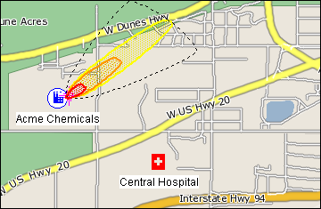
Figure 5.1: An ALOHA threat zone plot. The red, orange, and yellow zones indicate areas where specific Level of Concern thresholds are exceeded.
You can see that the depiction of the plume is very smooth and symmetrical. This is because the model does not account for changes in wind direction or speed.
For predicting the dispersion of plumes from non-continuous releases and during changing or calm wind conditions, modified Gaussian models (called Puff Models) are used. More recently-developed models have parameterizations to improve the handling of stability, convection, mixing, and terrain effects. Limitations of Gaussian/Puff models still reside in the simplified treatment of the turbulence and the meteorology.
For more complex terrain and meteorological conditions, Lagrangian and Eulerian models are more appropriate. They also work well for homogeneous and stationary conditions over flat terrain.
Lagrangian Particle Models
In a Lagrangian particle model, the atmospheric transport and dispersion of pollutants
is simulated by a large number of small tracers called
The figure 5.2 is an example of the MLDPn model (Model Lagrangien de Dispersion de Particules). See EERs dispersion models.

Figure 5.2: Port_Lambton, Ontario. Near-surface relative concentration.
;)
In the plot, the colors indicate various levels of concentration. As one can see, the output looks a little more realistic in terms of the variability you would expect due to fluctuations in the wind.
Eulerian Models
An Eulerian dispersion model is similar to a Lagrangian model in that it can also simulate the movement of a pollutant released from a source.
The main difference between the two models is that the Eulerian models use a fixed three-dimensional grid as a frame of reference rather than a
moving frame of reference.
In a Lagrangian model, an observer follows along with the parcels that represent the plume. In an Eulerian model, the observer
watches the plume go by at a point fixed in space.
These Lagrangian / Eulerian models can be applied for long/mid/near field and for long/short-range simulations. These models perform best when they are driven by
a detailed (prognostic) meteorological model.
For the Eulerian approach, the size of the grid cells employed limits the accuracy of the dispersion. Undesirable artificial dispersion associated with numerical
integration of the advection equation exists. This can lead
to appreciable numerical errors especially near the source when the latter is not resolved by the grid.
The Lagrangian approach has the advantage of permitting a better representation of the source when it is of a small scale.
On the other hand, in areas far from a source, representation of the plume by Lagrangian particles can be inefficient due to the
large number of particles required to achieve a smooth characterization of the concentration. An insufficient number of particles
leads to greater error on concentration predictions. However, using a large number of particles leads to longer calculation times. The amount
of computer memory may also limit calculation times. In such cases, an Eulerian approach is preferable.
Lagrangian / Eulerian ATMs produce better results than simple Gaussian models because they use more realistic winds, variable in space and evolving in time. However, they require more expertise and computer power to run.
As is the case for Gaussian models, most operational Lagrangian / Eulerian models do not take into account the complex wind structures associated with buildings in cases of high densely built-up areas with complex geometry.
Small-scale Urban Dispersion Models
This type of model resolves the wind around building at greater levels of detail. Computational Fluid Dynamics (CFD) models are a type of small-scale model used to simulate the complex flow patterns created in urban areas by large buildings and street canyons. CFD modeling is currently a very active area of research and development. These models are particularly valuable for predicting transport and diffusion in urban environments. The figure 5.3 shows an example of such a model.
Figure 5.3: Example of the relative concentration at the ground in an urban area, modeled by the CUDM system.
<< Previous | >> Next